Deep Neural Network for Image Classification: Application

Build your cat/not-a-cat classifier.

Problem Statement

• Build and train a deep L-layer neural network, and apply it to supervised learning

Packages

import time
import numpy as np
import h5py
import matplotlib.pyplot as plt
import scipy
from PIL import Image
from scipy import ndimage
from dnn_app_utils_v3 import *
from public_tests import *

%matplotlib inline
plt.rcParams['figure.figsize'] = (5.0, 4.0) # set default size of plots
plt.rcParams['image.interpolation'] = 'nearest'
plt.rcParams['image.cmap'] = 'gray'

%load_ext autoreload
%autoreload 2

np.random.seed(1)

Load and Process the Dataset

You’ll be using the same “Cat vs non-Cat” dataset as in “Logistic Regression as a Neural Network” (Assignment 2). The model you built back then had 70% test accuracy on classifying cat vs non-cat images. Hopefully, NN model will perform even better!

Problem Statement: You are given a dataset (“data.h5”) containing: - a training set of m_train images labelled as cat (1) or non-cat (0) - a test set of m_test images labelled as cat and non-cat - each image is of shape (num_px, num_px, 3) where 3 is for the 3 channels (RGB).

Let’s get more familiar with the dataset. Load the data from the cell below.

train_x_orig, train_y, test_x_orig, test_y, classes = load_data()

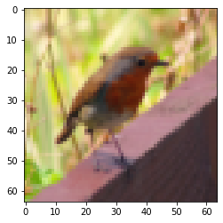
The following code will show you an image in the dataset. Feel free to change the index and re-run the cell multiple times to check out other images.

# Example of a picture
index = 10
plt.imshow(train_x_orig[index])
print ("y = " + str(train_y[0,index]) + ". It's a " + classes[train_y[0,index]].decode("utf-8") +  " picture.")

y = 0. It's a non-cat picture.

train_x_orig[index].shape

(64, 64, 3)

# Explore your dataset 
m_train = train_x_orig.shape[0]
num_px = train_x_orig.shape[1]
m_test = test_x_orig.shape[0]

print ("Number of training examples: " + str(m_train))
print ("Number of testing examples: " + str(m_test))
print ("Each image is of size: (" + str(num_px) + ", " + str(num_px) + ", 3)")
print ("train_x_orig shape: " + str(train_x_orig.shape))
print ("train_y shape: " + str(train_y.shape))
print ("test_x_orig shape: " + str(test_x_orig.shape))
print ("test_y shape: " + str(test_y.shape))

Number of training examples: 209
Number of testing examples: 50
Each image is of size: (64, 64, 3)
train_x_orig shape: (209, 64, 64, 3)
train_y shape: (1, 209)
test_x_orig shape: (50, 64, 64, 3)
test_y shape: (1, 50)

As usual, you reshape and standardize the images before feeding them to the network. The code is given in the cell below.

# Reshape the training and test examples 
train_x_flatten = train_x_orig.reshape(train_x_orig.shape[0], -1).T   # The "-1" makes reshape flatten the remaining dimensions
test_x_flatten = test_x_orig.reshape(test_x_orig.shape[0], -1).T

# Standardize data to have feature values between 0 and 1.
train_x = train_x_flatten/255.
test_x = test_x_flatten/255.

print ("train_x's shape: " + str(train_x.shape))
print ("test_x's shape: " + str(test_x.shape))

train_x's shape: (12288, 209)
test_x's shape: (12288, 50)

Note: \(12,288\) equals \(64 \times 64 \times 3\), which is the size of one reshaped image vector.

Model Architecture

2-layer Neural Network

Now that you’re familiar with the dataset, it’s time to build a deep neural network to distinguish cat images from non-cat images!

Build two different models:

• A 2-layer neural network
• An L-layer deep neural network

Then, you’ll compare the performance of these models, and try out some different values for \(L\).

Let’s look at the two architectures:

Detailed Architecture of Figure 2: - The input is a (64,64,3) image which is flattened to a vector of size \((12288,1)\). - The corresponding vector: \([x_0,x_1,...,x_{12287}]^T\) is then multiplied by the weight matrix \(W^{[1]}\) of size \((n^{[1]}, 12288)\). - Then, add a bias term and take its relu to get the following vector: \([a_0^{[1]}, a_1^{[1]},..., a_{n^{[1]}-1}^{[1]}]^T\). - Multiply the resulting vector by \(W^{[2]}\) and add the intercept (bias). - Finally, take the sigmoid of the result. If it’s greater than 0.5, classify it as a cat.

L-layer Deep Neural Network

General Methodology

As usual, follow the Deep Learning methodology to build the model:

1. Initialize parameters / Define hyperparameters
2. Loop for num_iterations:
   
   1. Forward propagation
      
   2. Compute cost function
      
   3. Backward propagation
      
   4. Update parameters (using parameters, and grads from backprop)
3. Use trained parameters to predict labels

Now go ahead and implement those two models!

Two-layer Neural Network

two_layer_model

Use the helper functions you have implemented in the previous assignment to build a 2-layer neural network with the following structure: LINEAR -> RELU -> LINEAR -> SIGMOID. The functions and their inputs are:

def initialize_parameters(n_x, n_h, n_y):
    ...
    return parameters 
def linear_activation_forward(A_prev, W, b, activation):
    ...
    return A, cache
def compute_cost(AL, Y):
    ...
    return cost
def linear_activation_backward(dA, cache, activation):
    ...
    return dA_prev, dW, db
def update_parameters(parameters, grads, learning_rate):
    ...
    return parameters

### CONSTANTS DEFINING THE MODEL ####
n_x = 12288     # num_px * num_px * 3
n_h = 7
n_y = 1
layers_dims = (n_x, n_h, n_y)
learning_rate = 0.0075

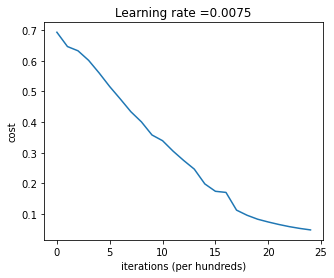
def two_layer_model(X, Y, layers_dims, learning_rate = 0.0075, num_iterations = 3000, print_cost=False):
    """
    Implements a two-layer neural network: LINEAR->RELU->LINEAR->SIGMOID.
    
    Arguments:
    X -- input data, of shape (n_x, number of examples)
    Y -- true "label" vector (containing 1 if cat, 0 if non-cat), of shape (1, number of examples)
    layers_dims -- dimensions of the layers (n_x, n_h, n_y)
    num_iterations -- number of iterations of the optimization loop
    learning_rate -- learning rate of the gradient descent update rule
    print_cost -- If set to True, this will print the cost every 100 iterations 
    
    Returns:
    parameters -- a dictionary containing W1, W2, b1, and b2
    """
    
    np.random.seed(1)
    grads = {}
    costs = []                              # to keep track of the cost
    m = X.shape[1]                           # number of examples
    (n_x, n_h, n_y) = layers_dims
    
    parameters = initialize_parameters(n_x, n_h, n_y)
    
    # Get W1, b1, W2 and b2 from the dictionary parameters.
    W1 = parameters["W1"]
    b1 = parameters["b1"]
    W2 = parameters["W2"]
    b2 = parameters["b2"]
    
    # Loop (gradient descent)

    for i in range(0, num_iterations):
        A1, cache1 = linear_activation_forward(X, W1, b1, activation='relu')
        A2, cache2 = linear_activation_forward(A1, W2, b2, activation='sigmoid')
        cost = compute_cost(A2, Y)
        
        # Initializing backward propagation
        dA2 = - (np.divide(Y, A2) - np.divide(1 - Y, 1 - A2))
        
        # Backward propagation. Inputs: "dA2, cache2, cache1". Outputs: "dA1, dW2, db2; also dA0 (not used), dW1, db1".
        dA1, dW2, db2 = linear_activation_backward(dA2, cache2, activation='sigmoid')
        dA0, dW1, db1 = linear_activation_backward(dA1, cache1, activation='relu')
        
        # Set grads['dWl'] to dW1, grads['db1'] to db1, grads['dW2'] to dW2, grads['db2'] to db2
        grads['dW1'] = dW1
        grads['db1'] = db1
        grads['dW2'] = dW2
        grads['db2'] = db2
        parameters = update_parameters(parameters, grads, learning_rate)

        # Retrieve W1, b1, W2, b2 from parameters
        W1 = parameters["W1"]
        b1 = parameters["b1"]
        W2 = parameters["W2"]
        b2 = parameters["b2"]
        
        # Print the cost every 100 iterations
        if print_cost and i % 100 == 0 or i == num_iterations - 1:
            print("Cost after iteration {}: {}".format(i, np.squeeze(cost)))
        if i % 100 == 0 or i == num_iterations:
            costs.append(cost)

    return parameters, costs

def plot_costs(costs, learning_rate=0.0075):
    plt.plot(np.squeeze(costs))
    plt.ylabel('cost')
    plt.xlabel('iterations (per hundreds)')
    plt.title("Learning rate =" + str(learning_rate))
    plt.show()

parameters, costs = two_layer_model(train_x, train_y, layers_dims = (n_x, n_h, n_y), num_iterations = 2, print_cost=False)

print("Cost after first iteration: " + str(costs[0]))

two_layer_model_test(two_layer_model)

Cost after iteration 1: 0.6926114346158595
Cost after first iteration: 0.693049735659989
Cost after iteration 1: 0.6915746967050506
Cost after iteration 1: 0.6915746967050506
Cost after iteration 1: 0.6915746967050506
Cost after iteration 2: 0.6524135179683452
 All tests passed.

Train the model

If your code passed the previous cell, run the cell below to train your parameters.

• The cost should decrease on every iteration.

• It may take up to 5 minutes to run 2500 iterations.

parameters, costs = two_layer_model(train_x, train_y, layers_dims = (n_x, n_h, n_y), num_iterations = 2500, print_cost=True)
plot_costs(costs, learning_rate)

Cost after iteration 0: 0.693049735659989
Cost after iteration 100: 0.6464320953428849
Cost after iteration 200: 0.6325140647912677
Cost after iteration 300: 0.6015024920354665
Cost after iteration 400: 0.5601966311605747
Cost after iteration 500: 0.5158304772764729
Cost after iteration 600: 0.4754901313943325
Cost after iteration 700: 0.43391631512257495
Cost after iteration 800: 0.4007977536203886
Cost after iteration 900: 0.3580705011323798
Cost after iteration 1000: 0.3394281538366413
Cost after iteration 1100: 0.30527536361962654
Cost after iteration 1200: 0.2749137728213015
Cost after iteration 1300: 0.2468176821061484
Cost after iteration 1400: 0.19850735037466102
Cost after iteration 1500: 0.17448318112556638
Cost after iteration 1600: 0.1708076297809692
Cost after iteration 1700: 0.11306524562164715
Cost after iteration 1800: 0.09629426845937156
Cost after iteration 1900: 0.0834261795972687
Cost after iteration 2000: 0.07439078704319085
Cost after iteration 2100: 0.06630748132267933
Cost after iteration 2200: 0.05919329501038172
Cost after iteration 2300: 0.053361403485605606
Cost after iteration 2400: 0.04855478562877019
Cost after iteration 2499: 0.04421498215868956

Nice! You successfully trained the model. Good thing you built a vectorized implementation! Otherwise it might have taken 10 times longer to train this.

Now, you can use the trained parameters to classify images from the dataset. To see your predictions on the training and test sets, run the cell below.

predictions_train = predict(train_x, train_y, parameters)

Accuracy: 0.9999999999999998

predictions_test = predict(test_x, test_y, parameters)

Accuracy: 0.72

It seems that your 2-layer neural network has better performance (72%) than the logistic regression implementation (70%). Let’s see if you can do even better with an \(L\)-layer model.

Note: You may notice that running the model on fewer iterations (say 1500) gives better accuracy on the test set. This is called “early stopping” and you’ll hear more about it in the next course. Early stopping is a way to prevent overfitting.

L-layer Neural Network

L_layer_model

Use the helper functions you implemented previously to build an \(L\)-layer neural network with the following structure: [LINEAR -> RELU]\(\times\)(L-1) -> LINEAR -> SIGMOID. The functions and their inputs are:

def initialize_parameters_deep(layers_dims):
    ...
    return parameters 
def L_model_forward(X, parameters):
    ...
    return AL, caches
def compute_cost(AL, Y):
    ...
    return cost
def L_model_backward(AL, Y, caches):
    ...
    return grads
def update_parameters(parameters, grads, learning_rate):
    ...
    return parameters

### CONSTANTS ###
layers_dims = [12288, 20, 7, 5, 1] #  4-layer model

def L_layer_model(X, Y, layers_dims, learning_rate = 0.0075, num_iterations = 3000, print_cost=False):
    """
    Implements a L-layer neural network: [LINEAR->RELU]*(L-1)->LINEAR->SIGMOID.
    
    Arguments:
    X -- input data, of shape (n_x, number of examples)
    Y -- true "label" vector (containing 1 if cat, 0 if non-cat), of shape (1, number of examples)
    layers_dims -- list containing the input size and each layer size, of length (number of layers + 1).
    learning_rate -- learning rate of the gradient descent update rule
    num_iterations -- number of iterations of the optimization loop
    print_cost -- if True, it prints the cost every 100 steps
    
    Returns:
    parameters -- parameters learnt by the model. They can then be used to predict.
    """

    np.random.seed(1)
    costs = []                         # keep track of cost
    
    parameters = initialize_parameters_deep(layers_dims)
    # Loop (gradient descent)
    for i in range(0, num_iterations):

        # Forward propagation: [LINEAR -> RELU]*(L-1) -> LINEAR -> SIGMOID
        AL, caches = L_model_forward(X, parameters)

        # Compute cost
        cost = compute_cost(AL, Y)
    
        # Backward propagation
        grads = L_model_backward(AL, Y, caches)
 
        # Update parameters
        parameters = update_parameters(parameters, grads, learning_rate)
                
        # Print the cost every 100 iterations
        if print_cost and i % 100 == 0 or i == num_iterations - 1:
            print("Cost after iteration {}: {}".format(i, np.squeeze(cost)))
        if i % 100 == 0 or i == num_iterations:
            costs.append(cost)
    
    return parameters, costs

parameters, costs = L_layer_model(train_x, train_y, layers_dims, num_iterations = 1, print_cost = False)

print("Cost after first iteration: " + str(costs[0]))

L_layer_model_test(L_layer_model)

Cost after iteration 0: 0.7717493284237686
Cost after first iteration: 0.7717493284237686
Cost after iteration 1: 0.7070709008912569
Cost after iteration 1: 0.7070709008912569
Cost after iteration 1: 0.7070709008912569
Cost after iteration 2: 0.7063462654190897
 All tests passed.

Train the model

If your code passed the previous cell, run the cell below to train your model as a 4-layer neural network.

• The cost should decrease on every iteration.

• It may take up to 5 minutes to run 2500 iterations.

parameters, costs = L_layer_model(train_x, train_y, layers_dims, num_iterations = 2500, print_cost = True)

Cost after iteration 0: 0.7717493284237686
Cost after iteration 100: 0.6720534400822914
Cost after iteration 200: 0.6482632048575212
Cost after iteration 300: 0.6115068816101356
Cost after iteration 400: 0.5670473268366111
Cost after iteration 500: 0.5401376634547801
Cost after iteration 600: 0.5279299569455267
Cost after iteration 700: 0.4654773771766851
Cost after iteration 800: 0.369125852495928
Cost after iteration 900: 0.39174697434805344
Cost after iteration 1000: 0.31518698886006163
Cost after iteration 1100: 0.2726998441789385
Cost after iteration 1200: 0.23741853400268137
Cost after iteration 1300: 0.19960120532208644
Cost after iteration 1400: 0.18926300388463307
Cost after iteration 1500: 0.16118854665827753
Cost after iteration 1600: 0.14821389662363316
Cost after iteration 1700: 0.13777487812972944
Cost after iteration 1800: 0.1297401754919012
Cost after iteration 1900: 0.12122535068005211
Cost after iteration 2000: 0.11382060668633713
Cost after iteration 2100: 0.10783928526254133
Cost after iteration 2200: 0.10285466069352679
Cost after iteration 2300: 0.10089745445261786
Cost after iteration 2400: 0.09287821526472398
Cost after iteration 2499: 0.08843994344170202

pred_train = predict(train_x, train_y, parameters)

Accuracy: 0.9856459330143539

pred_test = predict(test_x, test_y, parameters)

Accuracy: 0.8

It seems that your 4-layer neural network has better performance (80%) than your 2-layer neural network (72%) on the same test set.

This is pretty good performance for this task.

To obtain even higher accuracy systematically search for better hyperparameters: learning_rate, layers_dims, or num_iterations, for example.

Results Analysis

First, take a look at some images the L-layer model labeled incorrectly. This will show a few mislabeled images.

print_mislabeled_images(classes, test_x, test_y, pred_test)

A few types of images the model tends to do poorly on include: - Cat body in an unusual position - Cat appears against a background of a similar color - Unusual cat color and species - Camera Angle - Brightness of the picture - Scale variation (cat is very large or small in image)

References

• for auto-reloading external module

• https://www.coursera.org/learn/neural-networks-deep-learning/programming/Sfu8g/deep-neural-network-application/lab?path=%2Fnotebooks%2Frelease%2FW4A2%2FDeep%2520Neural%2520Network%2520-%2520Application.ipynb